Data Assimilation
Introduction
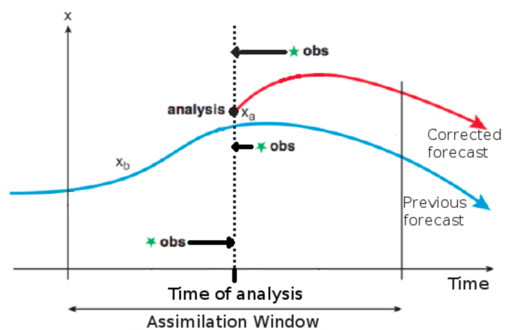
Data Assimilation (DA) is the art of combining information from different sources in an optimal way. In climate and NWP, these sources are a first guess and observations with the aim of improving an estimate of the state of a system. DA has two main objectives.
1) Produce an initial state from which we can start our forecast. 2) Quantifying the uncertainty of the initial state.
From the initial state of the atmosphere the model integrates a set of prognostic equations forward in time. This is prediction.
What is the optimal/best analysis in operational NWP?
- The best analysis is the one that leads to the best forecast, not necessarily the analysis closest to the true state.
- Computational efficient: Depending on operational setup you should make your analysis in 30-60 minutes. Even your smartphones can compute a reasonable weather forecast faster than the weather evolves.
- Minimises error/maximises probability.
Jargon in DA
Our prior information is a First Guess (\(\mathbf{x_g}\)) and some Observations (\(\mathbf{y}\)). \(\mathbf{x_g}\) is the prior information and can for example be:
- A random guess (bad choice!)
- A climatological field (better, but room for improvement)
- The analysis from a previous cycle ∗ A short term forecast from the previous cycle \(\mathbf{x_b}\)
- Most often \(\mathbf{x_g}=\mathbf{x_b}\) in operational setups.
We shall refer to a short term forecast as the background field \(\mathbf{x_b}\), and denote our analysis as \(\mathbf{x_a}\)
Observation coverage/density
The DMI Harmonie model, "NEA", has about \(10^9\) prognostic variables that we need to assign an initial value to produce a forecast. We have far less observations (\(\approx 10^4\) to \(10^6\)) giving rise to an insufficient data coverage. Furthermore, observations are:
- Not evenly distributed in space and time
- Not taken exactly at the grid points.
- Not perfect - they contain errors. Quality control is needed.
An observation operator is needed to interpolate and convert to state variables if needed.
A refresher on statistics
Suppose we have the noon-day pressure \(p_i\) and temperature \(T_i\) at Copenhagen, every day for a year. Let \(n=365\). The mean pressure, \(\overline{p}\), is defined to be
and similarly for the mean temperature \(\overline{T}\).
The variance of pressure, \(\sigma_p^2\), is defined as
and similarly for variance of the temperature \(\sigma_T^2\).
The standard deviations, \(\sigma_p\) and \(\sigma_T\) are the square roots of the variances. They measure the root mean square deviation from the mean.
Framework of DA
As has been described we have information both from a short term forecast, \(\mathbf{x_b}\), and some observations \(\mathbf{y}\). We need to develop a framework for combining the two sources of information.
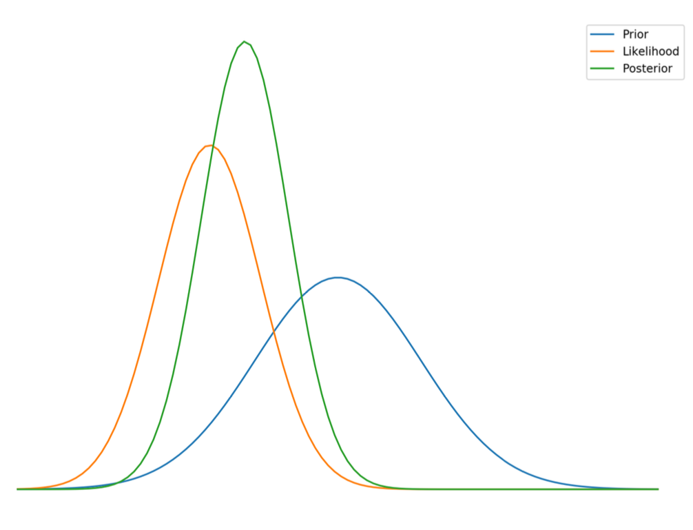
Luckily this framework already exist! → Bayes Theorem
- \(\text{pdf}(\mathbf{x}|\mathbf{y})\) is the posterior probability density function (pdf) of \(\mathbf{x}\) given \(\mathbf{y}\)
- \(\text{pdf}(\mathbf{y}|\mathbf{x})\) is the likelihood function, the \(\text{pdf}\) of the observations given the state variables.
- \(\text{pdf}(\mathbf{x})\) is the prior \(\text{pdf}\) of the state variables coming from the background field (model)
- \(\text{pdf}(\mathbf{y})\) is the evidence. It is used as a normalisation constant and often not computed explicitly so we will ignore this for now.
Combining information in the form of the prior and the likehood gives us a more narrow posterior \(\text{pdf}\). Note that as long one knows the associated error of either the model or observations the posterior will always gain information.
Reality bites
Making no approximations - considering the full non-linear DA problem - we have to find the joint \(\text{pdf}\) of all variables, that is the probabilities for all possible combinations of all of our variables.
Assume we only need 10 bins for each variable to generate a joint \(\text{pdf}\) and assume we have a small model of only \(10^6\) variables. Then we need to store \(10^{1000000}\) numbers.
There are approximately \(10^{80}\) atoms in the universe1. So data assimilation is much larger than the universe! We need \(10^{52}\) solar system sized hard drives to store just a googol (\(10^{100}\)) bytes, but we only have about \(10^{24}\) stars2. Approximations and optimisations are indeed needed.
The key here is that we can’t determine the pdf’s in large dimensional systems.
Approximate solutions
Estimating the \(\text{pdf}\)’s in large dimensional systems, such as in NWP, is practically impossible!
Approximate solutions of Bayes theorem leads to data assimilation methods.
- Variational methods: Solves for the mode of the posterior pdf.
- Kalman-based methods: Solves for the mean and covariance of posterior pdf.
- Particle Filters: Finds a sample representaion of the posterior pdf.
Variational methods and Kalman-based methods both assume errors to be Gaussian. Particle Filters, however have no such assumptions.
Variational Methods
The variational methods assume errors to be Gaussian. This is convenient as the pdf is completely determined by the mean and covariance. But it is also a strong constraint. Do the errors, in fact, follow a Gaussian?
In geophysics, we often deal with only the positive real axis, where we then often find a tail on the error distribution. For example precipitation, wind, salinity etc.
Let us see how the variational approach works with a scalar example of temperature observations.
We will feed our own ”toy data assimilation system” the observations, to obtain the most likely temperature given your observations.
The cost function
We assume that your observations has been drawn from a Gaussian distribution.
and likewise for \(T_2\). We can express the joint probability by multiplying the two probabilities together.
This is the same as the likelihood for \(T\) given \(T_1\) and \(T_2\), \(L(T|T_1,T_2)\). To find the most likely \(T\), which will be our analysis temperature \(T_a\), we want to maximise the likelihood given \(T_1\) and \(T_2\).
To make things easier, we take the logarithmic of this expression. Note that the logarithmic is a monotonic function, so maximising the logarithmic of the function is equivalent to maximising the function itself.
Note that maximising the function is equivalent to minimising the last term on the right-hand-side. For our ”two-temperature-problem” this is defined as our cost function.
Minimising \(J\) corresponds to maximising the likelihood of \(T\) given \(T_1\) and \(T_2\).
To minimise \(J\) to find our analysis temperature using the variational approach, we will start by guessing some value of \(T\) and explore space. Different algorithms exist for this such as "steepest-descent".
Example
"""
'Toy-Tool' to play with a very simple scalar case of the cost function
in variational data assimilation.

Given two guesses of temperature, we try to find the most likely
true temperature by minimizing a cost function.
"""

import numpy as np
import matplotlib.pyplot as plt

# Define variables
T1 = 21.6  # First guess of temperature
sigma1 = 1.8  # Standard deviation for T1

T2 = 23.4  # Second guess of temperature
sigma2 = 0.8  # Standard deviation for T2

# Initial guess (mean of T1 and T2)
T0 = (T1 + T2) / 2

# Initialize variables
T = T0  # Current temperature guess
eps = 0.1  # Epsilon for perturbation
J0 = 2000.  # Initial cost value

# Lists to store iteration data
iteration = []
Ta = []
costF = []

# Perform 100 iterations
for k in range(100):
    direction = np.random.randint(-1, 2) + eps
    size_direction = np.random.rand(1) * direction

    Tg = T + size_direction  # New temperature guess
    J = 1/2 * ((Tg - T1)**2 / sigma1**2 + (Tg - T2)**2 / sigma2**2)  # Cost function

    # Update if new cost is lower
    if J < J0 and k > 0:
        J0 = J
        T = Tg
        iteration.append(k)
        Ta.append(T)
        costF.append(J)
        print(T, J)

# Plotting
fig = plt.figure()
plt.plot(Ta, iteration)
plt.gca().invert_yaxis()
plt.ylabel('Iteration')
plt.xlabel('T [C]')
plt.show()
Probability distributions for the multivariate case
The principles we have just seen, are the same in the multivariate case.
The prior
The likelihood
The posterior
Notation
\(\mathbf{x}\): State vector of size \(n\)
\(\mathbf{x_b}\): Background state vector of size \(n\)
\(\mathbf{P}_b\) or \(\mathbf{B}\): Background error covariance matrix of size \(n\times n\)
\(\mathbf{y}\): Observation vector of size \(p\)
\(\mathbf{R}\): Observation error covariance matrix of size \(p\times p\)
\(n\): Total number of grid points \(\times\) number of model variables (\(\approx 10^7\))
\(p\): Total number of observations (\(\approx 10^4\))
\(H(\mathbf{x})\): Observation operator that maps model space to observation space. \(H(x_i)\) is the models estimate on \(y_i\). \(H\) can be non-linear (eg. radiance measurements) or linear (eq. synop temperature measurements).
Cost function multivariate case
Taking the term in the brackets of the posterior gives us the cost function that we want to minimise to maximise the posterior.
where \(\mathbf{x}\) is the state vector with all variables. The \(\mathbf{x}\) that minimises the cost function, \(J\) is our analysis state vector \(\mathbf{x}_a\). \(\mathbf{P}_b\) is the background error covariance matrix. \(\mathbf{P}_b\) is sometimes also denoted \(\mathbf{B}\) in the literature. Here I use \(\mathbf{P}_b\) for consistency with the Kalman Filter algorithm (to be introduced)
The cost function cannot be computed directly. Different assumptions leads to either 3DVar or 4DVar.
\(\mathbf{P}_b\) is a huge matrix! (\(\approx 10^7\times10^7\)) - We can’t store this on a computer, so we are forced to simplify it. Furthermore, it is not given that we have all the information needed to determine all of its elements.
We dont know \(\mathbf{P}_b\). In general \(\mathbf{P}_b = \text{cov}[\mathbf{x}_t − \mathbf{x}_b]\), but we have no way to know \(\mathbf{x}_t\), therefore a proxy is needed for \(\mathbf{x}_t\).
As a proxy for \(\mathbf{x}_t\) one can use ”observation-minus-background” statistics, by running the model for a long period and see how the error looks in average.
\(\mathbf{P}_b\) is essential. Its role is to spread out information from observations. How should a pressure observation in Copenhagen affect variables in Oslo? Also, it ensures dynamically consistent increments in other model variables (How should a temperature increase affect the wind?)
Tip
Good To Know: \(\mathbf{P}_b\) is often referred to as ”structure functions” in the literature.
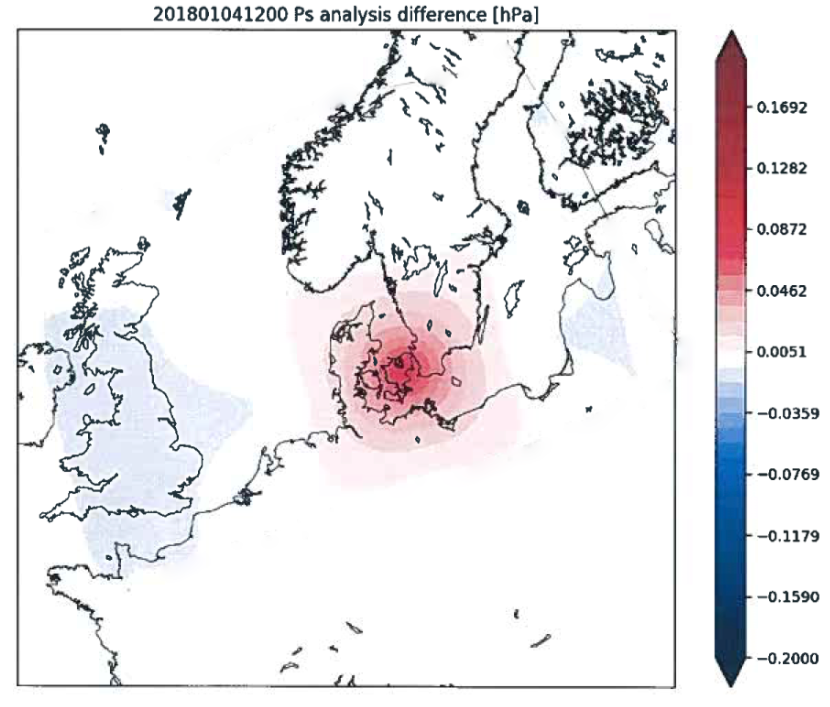
In the figure the difference (increment) between to analysis states is shown. A single additional pressure observation is assimilated in the second analysis. The increment is largest close to the observation and decreases with distance. The spread of the increment is determined by \(\mathbf{P}_b\).
Solving for the gradient of the cost function
The minimum of the cost function is obtained for \(\mathbf{x}=\mathbf{x}_a\), e.g. the solution of
So we wish to solve for the gradient of the cost function. To simplify the problem we linearise the observation operator \(H\) as
and assume that the analysis is close to the truth so that we can write
assuming \(\mathbf{x}-\mathbf{x}_b\) is small, \(\mathbf{y}-H(\mathbf{x})\) can be written as
This is an advantage as \(H(\mathbf{x}_b)\) and \(\mathbf{x}\) is known a priori. The cost function can now be written as
If we then assume that \(\mathbf{R}\) is symmetric so that \(\mathbf{HR}^{-1}=\mathbf{R}^{-1}\mathbf{H}\) and expanding the brackets we get
If we combine the first two terms we get
Given a quadratic function \(F(\mathbf{x})=\frac{1}{2}\mathbf{x}^T\mathbf{Ax}+\mathbf{d}^T\mathbf{x}+c\) the gradient is given by \(\nabla F(\mathbf{x})=\mathbf{Ax}+\mathbf{d}\). Using this and setting \(\nabla J(\mathbf{x})=0\) to ensure \(J\) is a minimum (though it could be a maximum or a saddle point) we obtain an analytical expression for the analysis state vector \(\mathbf{x}_a\).
The is the analytical solution to 3DVar. In practice it is solved by an iterative method such as the steepest descent method, as we saw in the scalar example. Unfortunately for us, it is impossible to invert such huge matrices as \(\mathbf{P}_b\) so we need to find approximations. Also 3DVar assumes all observations to be taken at the time of the analysis. This is not the case in reality. \(\mathbf{P}_b\) is also assumed to be constant in time, which is not the case in reality (not allowed to evolve dynamically).
Kalman-based Methods
Optimal Interpolation, Kalman Filter and Kalman Ensemble filters are methods that are widely used in operational centers and they are all based on the Kalman equations, which we shall derive to broaden our understanding of the methods.
An analysis is found by using a least square approach in the sense that we find an ’optimal’ analysis by minimising the errors.
We write our analysis \(\mathbf{x}_a\) as a linear combination of the background, \(\mathbf{x}_b\) and some observations \(\mathbf{y}\) as
where \(\mathbf{L}\) and \(\mathbf{W}\) are weights that we need to find.
One can derive the least square solution from this equation and at the same time get rid of one of the weights. This is a statistical approach trying to minimise the errors of the analysis.
The errors of \(\mathbf{x}_a\) and \(\mathbf{x}_b\) can be written as
where \(\mathbf{x}_t\) is the true (unknown) state. A linear observation process can be defined as
where \(\mathbf{H}\) is a matrix representing a linear transformation between the true variables into the observed ones (also called a forward operator) and \(\mathbf{b}_0\) is the observational error.
Assume that the observation error have zero mean and covariance \(\mathbf{R}\),
where \(\delta_{kk'}\) is the dirac-delta function.
Also assume that the observations errors and model errors are uncorrelated
Substitung the errors of the analysis and background into our analysis equation and subtracting \(\mathbf{x}_t\) we get
Assuming that the forecast error is unbiased (\(\mathbb{E}(\mathbf{e}_b)=\mathbb{E}(\mathbf{x}_b-\mathbf{x}_t)=0\)), the condition \((\mathbf{L}+\mathbf{WH}-\mathbf{I})\mathbb{E}(\mathbf{x}_t)=0\) must be met. In general \(\mathbb{E}(\mathbf{x}_t)\neq 0\) so to obtain an unbiased analysis we can write the first weight in terms of the second as
Substituting this into the analysis equation we get the Kalman analysis equation
Dimension
\(n=\text{Total number of grid points}\times\text{number of model variables}\)
\(\mathbf{x}\): State vector of size \(n\)
\(\mathbf{W}\): Weight matrix of size \(p\times n\) where \(p\) is the number of observations
\(\mathbf{y}\): Observation vector of size \(p\)
\(\mathbf{H}\): Matrix of size \(n\times p\)
Derivation of the weight
At this point \(\mathbf{W}\) is still unknown to us. \(\mathbf{W}\) chosen such that the variances are minimised. Consider the error covariance of the analysis,
Note that the variances are the trace of the error covariance matrix. This can be expanded by using the Kalman analysis equation and \(\mathbf{y}=\mathbf{Hx}_t+\mathbf{b}_0\) to get
This can be simplified by using the covariance matrix identity, \(\text{cov}(\mathbf{AB})=\mathbf{A}\text{cov}(\mathbf{B})\mathbf{A}^T\):
where \(\mathbf{P}_b=\text{cov}(\mathbf{x}_t-\mathbf{x}_b)\) and \(\mathbf{R}=\text{cov}(\mathbf{b}_0)\).
We expand by using that \(\mathbf{I}=\mathbf{I}^T\) and defining \(\mathbf{S}=\mathbf{HP}_b\mathbf{H}^T+\mathbf{R}\) to get
Recall that we want to minimise the trace of the error covariance matrix (to minimise the variances). We take the derivative of the trace of \(\mathbf{P}_a\) with respect to \(\mathbf{W}\) and setting it equal to 0 to find the minimum (hint: Use the matrix identity \(\nabla_A\text{Tr}(\mathbf{AB})=\mathbf{B}^T\)).
Using that \(\mathbf{P}_b\) is symetric (\(\mathbf{P}_b=\mathbf{P}_b^T\)) and solving for \(\mathbf{W}\) yields the optimal weight
This is called the Kalman gain and is the optimal weight that minimises the variances of the analysis.
Understanding the Kalman gain
It is important to get an intuitive understanding of the Kalman gain. The Kalman gain is a measure of how much we trust the observations. If the observation error is large, the Kalman gain will be small and vice versa. If the background error is large, the Kalman gain will be small and vice versa.
Recall that \(\mathbf{R}\) is the observational error covariance matrix and \(\mathbf{P}_b\) is the background error covariance matrix.
If the observational error is much larger than the model error the Kalman gain will go towards 0, making the innovation term in equation small, such that observations are given a low weight.
On the other hand, if the model error is much larger than the observational error the weight will go towards 1, given the innovation term a high weight in the analysis equation.
One advantage of the Kalman system is that we get the error of the analysis directly by computing \(\mathbf{P}_a\). This is not the case for the variational methods. However, we can now simplify the equation for \(\mathbf{P}_a\) by multiplying the Kalman gain with \(\mathbf{W}^T\mathbf{S}\) to get
Substituting this into the equation for \(\mathbf{P}_a\) we get
The Kalman filter and OI methods are very similar with some important differences though. In the Kalman Filter, \(\mathbf{P}_b\) is dynamic, hence updated with each analysis. In Optimal Interpolation (OI) \(\mathbf{P}_b\) is static, hence constant in time. Due to the dynamic \(\mathbf{P}_b\) in the Kalman Filter it is for example used partly in auto-piloting in airplanes and self-driving cars.
The Kalman Filter Algorithm
The Kalman Filter algorithm is a recursive algorithm which has a prediction step and an update step.
Prediction step
Update step
Here \(\mathbf{K}=\mathbf{W}\) is used for consistency with the literature. \(\mathbf{Q}\) is the forecast error covariance. \(\mathbf{M}\) is the linear tangent model and \(\mathbf{M}^T\) is its adjoint. \(\mathbf{M}\) is the operator that forwards the model in time from the analysis.
Optimal Interpolation (OI) equations
Analysis Equation:
Optimal Weight:
Analysis Error Covariance:
\(\mathbf{P}_b\) is static and is usually computed by running a model over a long period (weeks to months) and looking at the error statistics. Therefore \(\mathbf{P}_b\) must be updated for every change in model configuration (dynamics, physics, domain).
Characteristic overview of DA methods
| Method | Observations | Covariance | ||||
|---|---|---|---|---|---|---|
| Variational | Kalman | Sequential | Smoother | Static | Dynamic | |
| 3DVar | x | x | x | |||
| 4DVar | x | x | (x) | x | ||
| OI | x | x | x | |||
| KF | x | x | x |